1- Disclaimer
RhinoCentre Training Approach
This training module is part of a systematic series of training modules for the marine industry developed by RhinoCentre.About the author
 Gerard Petersen is naval architect, founder of RhinoCentre and uses Rhino since 2001 in his projects in the most integrated way. Petersen developed hull design and fairing skills to be able to develop innovative concepts with unique hull shapes like the integrated trimaran Kenau. The trimaran project proved that Rhino is a professional tool to turn an idea into reality. More and more, Petersen became convinced that Rhino is the perfect tool to model any vessel hull whether it is a ship, boat or yacht. The next step was to bring his developed knowledge and experience to a training. This way, anyone can profit from Rhino being a hull design and fairing tool. As Petersen offers Rhino training since 2005, he also has to experience how to transfer knowledge in a comprehensible way.
Training Videos of the exercises
 Naval architect Bas Goris created the training videos of the exercises 2-23. Petersen created the training videos 24-35.
Goris will also be one of the people who is assigned to give online training support for the 'Hull Design and Fairing' training modules. Goris developed the first ideas of the Rapid Hull Modeling Methodology in 2002. Then he shared this method with RhinoCentre which made it possible to continue its development.
Naval architect Bas Goris created the training videos of the exercises 2-23. Petersen created the training videos 24-35.
Goris will also be one of the people who is assigned to give online training support for the 'Hull Design and Fairing' training modules. Goris developed the first ideas of the Rapid Hull Modeling Methodology in 2002. Then he shared this method with RhinoCentre which made it possible to continue its development.
- Exercise 2-23 are made in Rhino 5.
- Exercise 24-35 are already made in Rhino 6 as it will be released in early 2018. As you will see, the look and feel of Rhino 6 is similar to Rhino 5. What will catch your eye mostly is that Rhino 6 shows the control points of curves when you select them.
- The videos of Exercise 24-35 are made at a resolution of 1920x1080 pixels.
- The videos of Exercise 2-23 are made at a lower resolution.
- The videos often zoom in and out to focus on the action of typing a command, turning on/off a layer etc. This is also done for those who watch these videos on a smaller screen like a tablet for example.
- The videos also often contain annotations that display the current action. For example arrows point out to look at another location than the position of the mouse pointer at that specific moment. Also often the use of specific keys on the keyboard are indicated. This might probably seem a bit stupid or unnecessary but this is also done for people who are deaf, have other hearing problems or find it difficult to understand the English pronunciation.
- We would like to hear your comments on the videos to be able to improve them.
About RhinoCentre
Since 2003 RhinoCentre shares and increases Rhino knowledge in offering training, consultancy and other services to the marine industry worldwide. The best example is the joined development of the Rapid Hull Modeling Methodology with people of several companies and organizations. On the other hand is RhinoCentre in close contact with McNeel & Associates, the developers of Rhino as well as plugin developers to make Rhino even better. RhinoCentre maintains with most of their customers a long lasting relationships based on trust and equality. Please contact us if you need any help regarding Rhino related issues.About the value of this training
We have invested more than a decade of experience in this training. To develop a training module like this one takes us at least three months. You and your company paid for this in time and money. Please keep this in mind in case you’re considering giving this training (or the associated training files) away, or even worse, publishing it on internet. There is no way we can prevent this with protections. Actually we don’t even want to try. We simply trust you on this.
|
3- How to learn Rhino
 Learning how to use commands and know how to find them again is the key to your success.
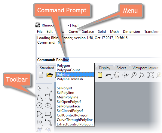
Most commands can be activated in four ways:
Learning how to use commands and know how to find them again is the key to your success.
Most commands can be activated in four ways:
- By typing them at the Command Prompt
- Via the Menu structure on top of the Rhino screen
- By clicking on an Icon in a Toolbar
- With an Alias (short cut)
When typing letters in the command prompt, Rhino presents all commands that contain these letters. This is a useful Rhino feature to find specific Rhino commands.
Rhino Command Help
[caption id="attachment_8666" align="alignright" width="688"]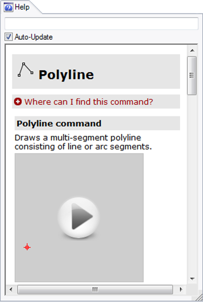 Fig.1: The CommandHelp panel[/caption]
Use the Rhino Command Help with Auto-Update (Fig.1) to teach you how a specific command works and where to find it.
Click the + to learn where to find a specific command in the menu or toolbars.
If the Command Help panel is not visible use the command _CommandHelp to show it.
Fig.1: The CommandHelp panel[/caption]
Use the Rhino Command Help with Auto-Update (Fig.1) to teach you how a specific command works and where to find it.
Click the + to learn where to find a specific command in the menu or toolbars.
If the Command Help panel is not visible use the command _CommandHelp to show it.
Rhino newsgroup & forum
If you get stuck with a problem post it on the Rhino user forum at: discourse.mcneel.com. Often within an hour you will get one or more answers from McNeel employees or other Rhino users. It is advised to send a Rhino file with the problem or add some screenshots.4- Before you start
To make sure the steps done in this manual are working as expected some standard settings are needed. Exercise 1: Before you start [video width="1280" height="720" mp4="https://www.rhinocentre.nl/wp-content/uploads/2017/10/Ex-01-Preparations.mp4"][/video]Exercise 1: Before you start[caption id="attachment_8667" align="alignnone" width="700"]
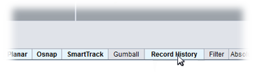
- Make sure 'Grid Snap' is turned off and 'Ortho', 'Osnap' and 'Planar' is turned on in the status bar (Fig.2)
Fig.2: Osnap toolbar & Status bar[/caption] [caption id="attachment_8662" align="alignright" width="412"]
Fig.3: Layer manager panel[/caption]
- Make sure that the Osnap toolbar is visible (Fig.2). If it’s not, go to 'Tools' > 'Object Snap' > and check 'Persistent Osnap Dialog'
- In the Osnap toolbar (Fig.2), turn on the following object snaps: 'End', 'Near', 'Point', 'Mid', 'Cen', 'Int'
- Make sure the Layer manager panel is visible (Fig.3). If it’s not, then run the _Layer command
- Download now the necessary training files: M1R1 - Training Files - Online
- Make sure to store the files in a secure place on your hard drive.
- Now copy the training files folder to the desktop. This makes it most easy to access the necessary files during the training.
- At last, create a new folder on your desktop and name it "WIP" (Work In Progress). In this folder you can save your training files thus keeping the original files clean.
Rhino viewport orientation
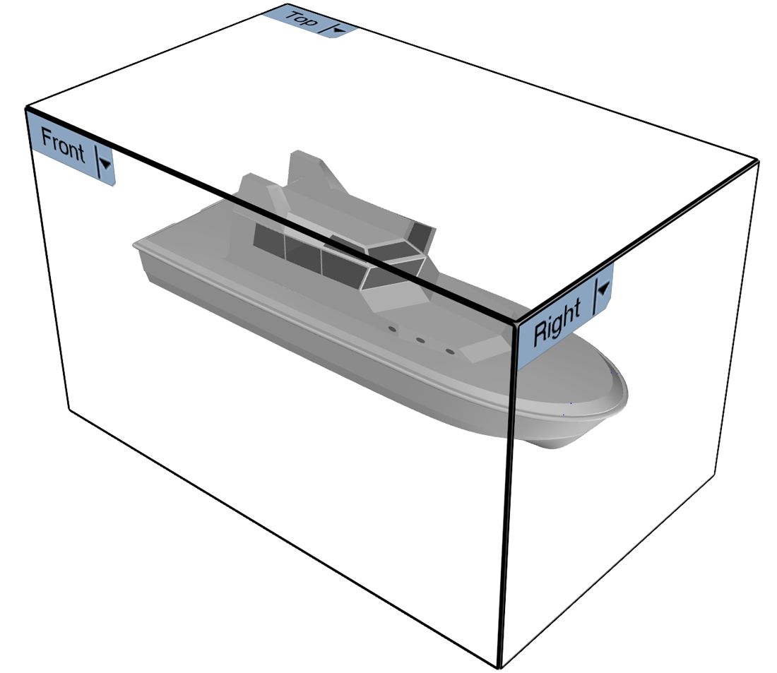 At this point one word about Rhino viewport orientation in Rhino. In naval architecture, the hull center line orientation is along the X-axis which is unfortunately inconsistent with the Rhino viewport setup because:
- The side view of the hull is called 'Front' in Rhino.
- The front view is called 'Right' in Rhino.
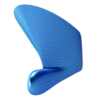
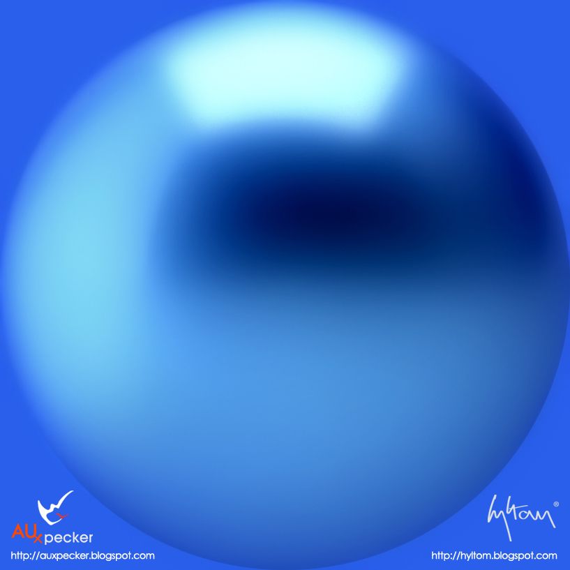 Fig. 4: Environment map image[/caption]
During freeform modeling of a hull, the surface quality is primarily judged by checking the reflection of the surface while rotating the model.
An "environment map" in rendered display offers the best visibility for that as bumps and hollows are best visible then.
Environment maps are spherical images with a certain color, gloss and reflection (Fig. 4: Environment map image). These images are projected on the objects to simulate a certain environment. They show the gloss and reflection of the environment map and not the real lighting setup in Rhino. In other words it is a trick to create a certain dynamic visual effect.
While editing the model you can instantly witness the changes in the reflection during rotating and zooming in and out of the model. Of course there are other ways to evaluate the exact size and shape of a surfaces like intersection curves at certain positions (which will get covered later in this course) but our first and most simple evaluation tool will be the a visual check using the "Glossy for Fairing" display mode.
Fig. 4: Environment map image[/caption]
During freeform modeling of a hull, the surface quality is primarily judged by checking the reflection of the surface while rotating the model.
An "environment map" in rendered display offers the best visibility for that as bumps and hollows are best visible then.
Environment maps are spherical images with a certain color, gloss and reflection (Fig. 4: Environment map image). These images are projected on the objects to simulate a certain environment. They show the gloss and reflection of the environment map and not the real lighting setup in Rhino. In other words it is a trick to create a certain dynamic visual effect.
While editing the model you can instantly witness the changes in the reflection during rotating and zooming in and out of the model. Of course there are other ways to evaluate the exact size and shape of a surfaces like intersection curves at certain positions (which will get covered later in this course) but our first and most simple evaluation tool will be the a visual check using the "Glossy for Fairing" display mode.

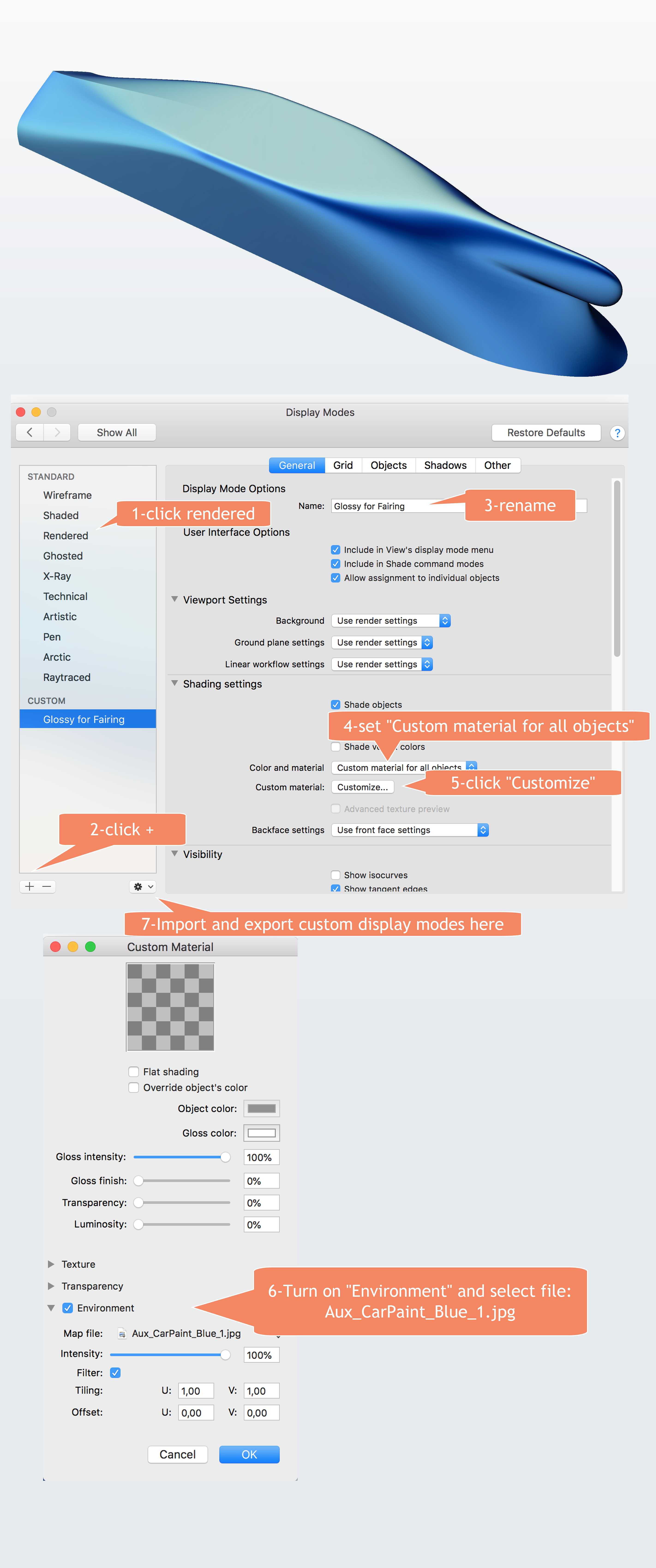 Fig.4.2: Rhino 6 for Mac - Glossy for Fairing Display.[/caption]
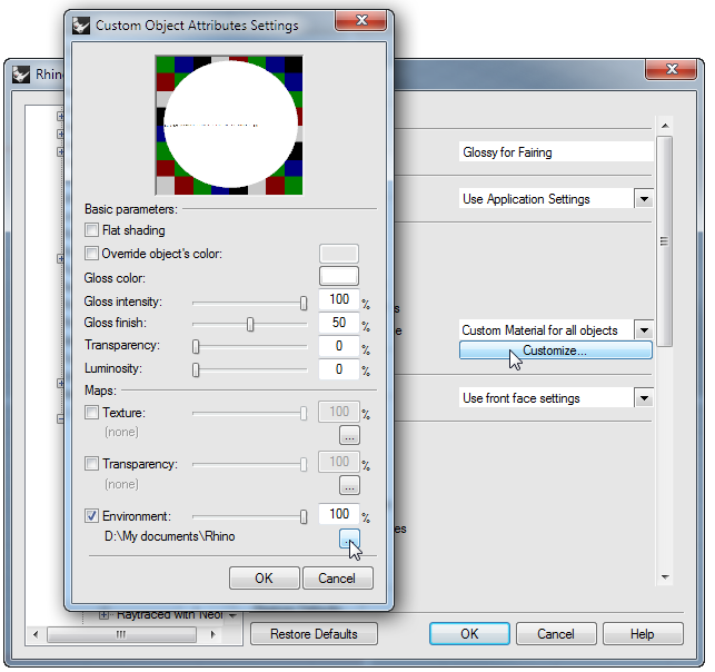 Fig. 5: Apply Custom Material[/caption]
 Fig. 6: Draw the first main frame curve[/caption]
 [caption id="attachment_9268" align="alignright" width="211"]
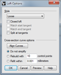 Fig. 7: Loft Options dialog[/caption]
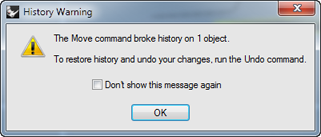 Fig. 8: History Warning[/caption]
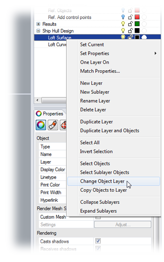 Fig. 9: Change Object Layer[/caption]
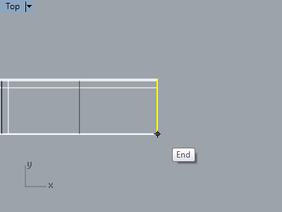 Fig. 10: Rotate the bow curve[/caption]
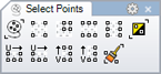
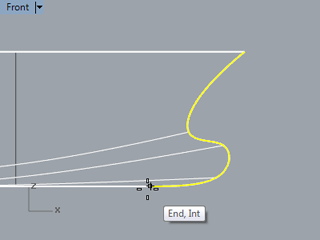 Fig. 11: Shear origin point[/caption]
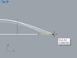 Fig. 12: Shear reference point[/caption]
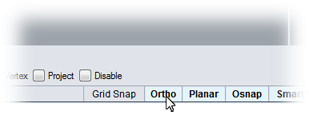 Fig. 13: Turn on Ortho[/caption]
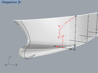 Fig. 14: X-ray display[/caption]
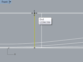 Fig. 15: Shear origin and reference point[/caption]
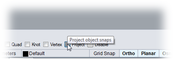 Fig. 16: Project object snaps[/caption]
 Fig. 17: Scale1D origin point[/caption]
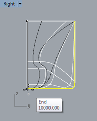 Fig. 18: Scale1D reference point[/caption]
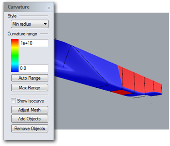 Fig. 19: The Curvature dialog[/caption]
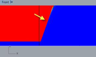 Fig. 20: Fore edge of the flat of side[/caption]
As you can see, the fore edge of the flat of side is more or less straight up (Fig. 20). Changing the shape and area of the flat of side is very simple by editing the loft curves.
For example:
Exercise 14-2: Edit the sixth loft curve
[video width="1920" height="1080" mp4="https://www.rhinocentre.nl/wp-content/uploads/2017/11/M1R1-Ex.-14-Part-2.mp4"][/video]
Fig. 20: Fore edge of the flat of side[/caption]
As you can see, the fore edge of the flat of side is more or less straight up (Fig. 20). Changing the shape and area of the flat of side is very simple by editing the loft curves.
For example:
Exercise 14-2: Edit the sixth loft curve
[video width="1920" height="1080" mp4="https://www.rhinocentre.nl/wp-content/uploads/2017/11/M1R1-Ex.-14-Part-2.mp4"][/video]
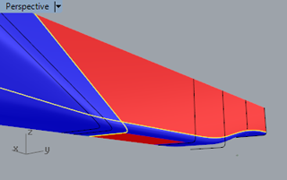 Fig. 21: ExtractIsocurve to get the edges of the flat of side[/caption]
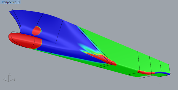 Fig. 22: Gaussian curvature display[/caption]
Notice that green areas are single curved, Red areas are spherical shaped. Blue areas are saddle shaped (hyperbolic).
Fig. 22: Gaussian curvature display[/caption]
Notice that green areas are single curved, Red areas are spherical shaped. Blue areas are saddle shaped (hyperbolic).
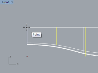 Fig. 23: Length Scale1D origin point[/caption]
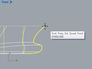 Fig. 24: Length Scale1D reference point[/caption]
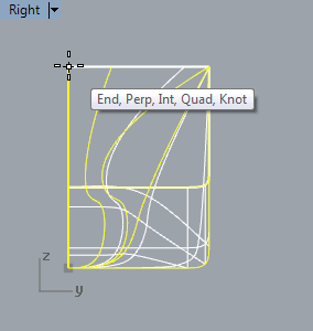 Fig. 25: Breadth Scale1D origin point[/caption]
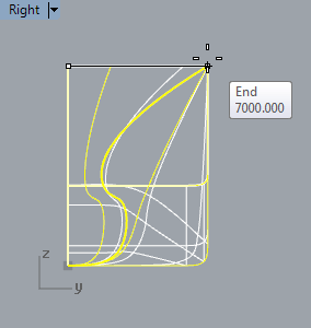 Fig. 26: Breadth Scale1D reference point[/caption]
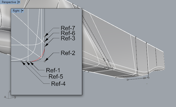 Fig. 27: Control points of all loft curves that contain the bilge radius[/caption]
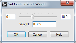 Fig. 28: Set Control Point Weight dialog[/caption]
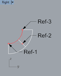 Fig. 29: Curvature Graph of an arc[/caption]
To analyze the shape of a curve or surface Rhino offers the curvature graph. This graph represents the second derivative of the mathematical function that describes the shape of the curve. There are a few typical characteristics that we will use in hull modeling:
Fig. 29: Curvature Graph of an arc[/caption]
To analyze the shape of a curve or surface Rhino offers the curvature graph. This graph represents the second derivative of the mathematical function that describes the shape of the curve. There are a few typical characteristics that we will use in hull modeling:
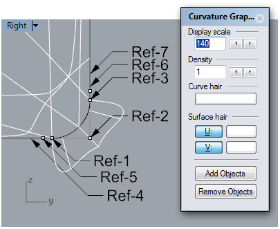 Fig. 30: The Curvature Graph dialog[/caption]
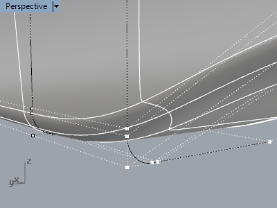 Fig. 31: Control points comparison[/caption]
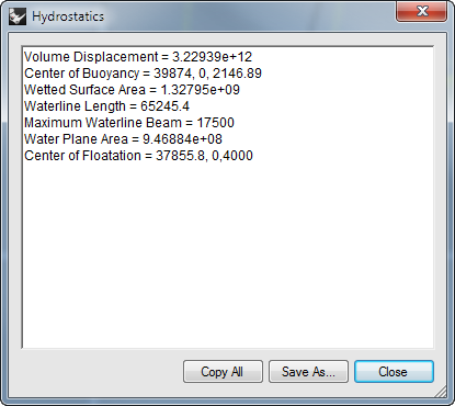 Fig. 32: Hydrostatics report[/caption]
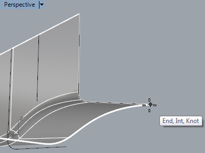 Fig. 33: First corner of plane[/caption]
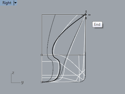 Fig. 34: Other corner of plane[/caption]
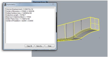
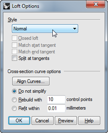 Fig. 35: Select "Normal" Loft style[/caption]
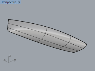 Fig. 36: Normal Loft[/caption]
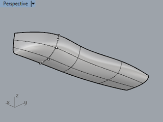 Fig. 37: Edit the additional curve[/caption]
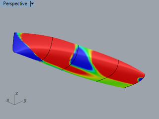 Fig. 38: Use CurvatureAnalysis to examine the result[/caption]
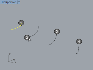 Fig. 39: Select the loft curves one by one[/caption]
 Fig. 40: Reverse the curve(s)[/caption]
9-Fairing techniques
When a hull is modeled based on loft curves, it is important to know some techniques that are used during fairing and editing a ship hull. The shape of the hull is edited by manipulating the shape and position of the loft curves. The shape of the curves is edited by moving its control points around. Before moving loft curves and control points they have to be selected in a clever way.Selecting objects in Rhino
In Rhino objects are selected over and over again. In order to edit a surface, curve or point it needs to be selected. As we don't know how experienced you already are with Rhino, we decided to show you some of the selection methods in Rhino. This ensures us that you know how to properly select objects in Rhino later in the course.- A single object can be selected by clicking on it.
- In case other objects are in vicinity, Rhino shows a selection dialog in which you can define which object has to be selected. A lot of trainees ignore this menu and click frantically on the object. Please use the selection menu to know for sure that you select the desired object. Another way is to find another viewport in which you can click directly on a single object. This is often the perspective viewport at a specific angle and zoomed in at the desired object location.
- Select multiple objects at once with a Window Selection (drag a selection rectangle from left to right) or Crossing Window Selection (drag a selection rectangle from right to left).
- To add objects to a selection press and hold the [Shift] key on the keyboard. Press and hold the [Ctrl] key to remove objects from a selection.
- Select objects of the same type by typing 'sel' in the command bar and notice the enormous amount of specific selections that can be executed
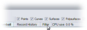 Fig. 41: Turn on / off Selection Filter[/caption]
- Since version 5 Rhino also offers very handy selection filters to restrict selections to a certain type. To open the dialog click Filter in the status bar (Fig. 41). It works similar to the persistent Osnap dialog:
- Left-click on a filter to turn it on / off
- Right-click on a filter to turn all others on / off
- [Shift] or [Ctrl] + left-click on a filter to turn all others off for just one time
Exercise 23: Selecting Objects by Picking, Window Selection and Crossing Window Selection [caption id="attachment_9241" align="alignright" width="320"]Fig. 42: Crossing Window Selection[/caption]
[caption id="attachment_9242" align="alignright" width="320"]
- Turn on the layers "Ship Hull Design > Loft Curves" and "Ship Hull Design > Loft Surface"
- Make sure both layers are unlocked
- Turn on layer "Exercise > Ref. Crossing Window Selection"
- In the "Top" viewport drag a selection window from A to B (right to left = Crossing Window Selection) (Fig. 42)
- Notice that two bow curves and the loft surface are selected.
- Press [Esc] or click somewhere in the top viewport (not on an object) to deselect all objects
- Lock layer "Ship Hull Design > Loft Surface"
- Again drag a selection window from A to B (just the two bow curves are selected)
Fig. 43: Toggle in the selection menu[/caption]
[caption id="attachment_9243" align="alignright" width="320"]
- Turn on their control points
- Click in the "Front" viewport on the control points at Ref-1 which define the bulb shape and notice the selection menu
- Move the mouse over one of the curve points in the selection menu (Fig. 43) and notice that one of the points in the "Top" viewport is displayed in white (Fig. 44)
- By moving over the other curve point in the selection menu the other point is displayed white
- This way it is possible to select one specific control point
- Click on 'None' in the selection menu to cancel the selection.
Fig. 44: Check in the Top viewport[/caption]
- In the "Front" viewport select the points at Ref-1 simultaneously with a window by dragging a selection window from left to right around the points
- Press and hold [Shift] on the keyboard and select the points at Ref-2 with a selectionwindow
- Notice in the perspective viewport that four control points have been selected now
- Extend the bulb by dragging the points forward. Even though the loft surface layer is locked, the surface updates due to record history
- Undo the dragging of the bulb control points
- Turn off layer "Exercise > Ref. Crossing Window Selection".
Moving control points to edit and fair loft curves
The position of curves and control points can be manipulated in several ways:- Dragging objects is the quickest way for rapid transformations which are more or less accurate;
- The Move command allows movements with a precise distance. It is not fast but very accurate;
- The Gumball is another way to move, rotate, scale, transform and copy objects in Rhino 5.0. It combines several editing commands in one clever manipulator.
- The Nudge feature is very useful for fairing purposes to move control points with a specific step size in a cumulative way using the arrow keys of the keyboard (you can adjust the nudge steps distance in the Rhino options > Modeling Aids > Nudge)
- Other useful Rhino tools:
[caption id="attachment_9244" align="alignright" width="318"]
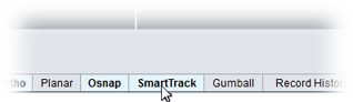 Fig. 45: Turn on / off SmartTrack[/caption]
- Using assist curves or 'SmartTrack' (Fig. 45) to align points
- Set XYZ coordinates to align several points at once to the same position in or/and X, Y, Z.
Due to a busy schedule of Bas Goris, the training videos in the rest of this training module were made by Gerard Petersen. These videos were also already made with Rhino 6 Beta. As you will see, there's not much difference in the look and feel. Most significant difference is that Rhino 6 shows instantly the control points of curves when you select them. The last difference is that these movies were made at a higher resolution of 1920x1080.Exercise 24: The Gumball [video width="1920" height="1080" mp4="https://www.rhinocentre.nl/wp-content/uploads/2017/11/M1R1-Ex.-24-Ger-R6.mp4"][/video]
Exercise 24: The Gumball [caption id="attachment_10413" align="alignright" width="333"]Fig. 46: Gumball[/caption]
- Turn on the Gumball Editor in the status bar at the bottom of the Rhino screen (Fig. 46).
- In the "Perspective" viewport, select the stern loft curve and notice the Gumball pops up.
- Move the curve a little forward by dragging the red arrow.
- Undo the movement.
[caption id="attachment_10414" align="alignnone" width="1498"]
- Click at the red arrow and type 2500 for the move distance.
- Undo the movement.
Fig. 47: New origin of Gumball[/caption]
[caption id="attachment_10412" align="alignnone" width="987"]
- In the "Front" viewport, select the two aft ship loft curves. Notice that the Gumball is displayed in between the two curves.
- Relocating the Gumball origin in the "Front" viewport:
- Press and hold [Ctrl] key on the keyboard and then click and hold the left mouse button.
- Now drag the gumball pivot point in the "Front" viewport a little bit upwards and still hold the left mouse button.
- Release the [Ctrl] key on the keyboard and still hold the left mouse button.
- Move the mouse pointer to the top of the hull and snap to the end point of the stern loft curve.
- Now release the left mouse button (Fig. 47).
- Now scale the two loft curves in Z-direction by moving the green open rectangle up and down.
- Undo the scaling.
Fig. 48: Rotate with Gumball[/caption]
- In the "Top" viewport, select the fourth loft curve from the stem.
- Make sure that 'Ortho' is turned off.
- Notice where the origin of the Gumball is located. Is it on the center line?
- If not, relocate the origin of the Gumball to the center line.
- Now use the blue arc to rotate the loft curve 30 degrees forward (in Top viewport) (Fig. 46).
- Take a look at the result.
- Undo the rotation.
- Turn off the Gumball in the status bar at the bottom of the Rhino screen
- At last press [F1] to open the Rhino help. Click at “Index” and type ‘Gumball’. Find out everything about Gumball functionality over here.
Nudge control point positions
Nudge makes it possible to move objects with a predefined step in a cumulative way. You can set the distance each nudge step will do in the Rhino options under Tools > Options > Modeling Aids > Nudge (Fig. 47). The settings have to be set according to the scale of the hull and the level of detail you are working at: Rough or refined. [caption id="attachment_9247" align="alignright" width="507"] Fig. 47: Nudge settings[/caption]
For this exercise set them to:
Fig. 47: Nudge settings[/caption]
For this exercise set them to:
- Nudge key alone: 10mm
- Ctrl+ Nudge key: 1mm
- Shift + Nudge key: 100mm
- Nudge direction: Use World Axes
“Use UVN” is very useful to move points in the normal direction of the surface at that point.Exercise 25: Nudge [video width="1920" height="1080" mp4="https://www.rhinocentre.nl/wp-content/uploads/2017/11/M1R1-Ex.-25-Ger-R6.mp4"][/video]
Exercise 25: Nudge [caption id="attachment_9248" align="alignright" width="415"]Fig. 48: Nudge key directions[/caption]
[caption id="attachment_9249" align="alignright" width="320"]
- Turn on the control points of the third loft curve from the bow
- Select the second to top control point
- Zoom in at this part of the ship in all viewports.
- Press the [^] Arrow key five times. See what's happening in the Right viewport. The movement is very small (5 x 10mm = 50mm)
- Read in the command history window on the top of the Rhino screen: Nudge 10.000, Cumulative 50.000
- Now also try this by pressing [^] Arrow key five times. Now the movement is larger (5 x 100mm = 500mm)
- Read in the command history window on the top of the Rhino screen: Nudge 100.000, Cumulative 550.000 (500 + 50 of the previous nudge)
Fig. 49: Evaluate the surface with glossiness[/caption]
- Press the [PageUp] or [Page Down] key for movements in the Z-direction
- Switch the perspective viewport display to 'Glossy for Fairing'
- Rotate the view in such a way that the white gloss is on the selected control point position (Fig. 49)
- Now play with nudge and notice the gloss appearance to get some feeling with Nudge
- Run _UndoMultiple and undo all Nudge steps
- Switch the perspective viewport display to 'Shaded' again.
Another way to quickly zoom in that area in all viewports is to select the two adjacent control points and run the macro: _Zoom _All _Selected. There is also a toolbar button for this macro and a menu entry: View > Zoom > Zoom Selected All. Of course this command also works if you just select one control point but then the zoom factor is very high.
Aligning Control Points
Quite often control points have to be aligned in one direction. This is also useful to create a planar bottom or flat of side when control points in these regions might have moved a little during fairing. The _SetPt command is very useful to align objects in the same X/Y/Z location. Exercise 26: Set XYZ Coordinates [video width="1920" height="1080" mp4="https://www.rhinocentre.nl/wp-content/uploads/2017/11/M1R1-Ex.-26-Ger-R6.mp4"][/video]Exercise 26: Set XYZ Coordinates [caption id="attachment_9250" align="alignright" width="133"]Fig. 50: Set Points dialog[/caption]
How to get this curve oriented straight up again? One way is to put all x-positions of the control points to the same value.
- Turn on the control points of the sixth loft curve (counted from the bow). This curve defines partly the forward shape of the flat of side.
- Select all control points of this loft curve and run _SetPt
- The 'Set Points' dialog pops up (Fig. 50). Check 'Set X' with the 'Align to World' option and press OK
- Now move the mouse in the "Front" viewport and watch the preview of the result. It is possible to click somewhere in between the adjacent curves, but in this case type an exact valuefor the X position: 35000
- Undo the SetPt operation. Then, turn off layer "Ship Hull Design".
Curvature Graph
[caption id="attachment_9251" align="alignnone" width="574"]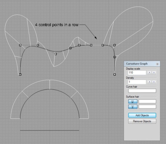 Fig. 51: Curvature graph[/caption]
The _CurvatureGraph command is an analysis tool that is used to examine the shape of a curve or surface.
We used it already when shaping the bilge radius. Now it’s time to explain the ins and outs with some exercises.
As mentioned before, the curvature graph shows the 2nd derivative of the mathematical function describing a curve.
The characteristics are shown in the image to the right (Fig. 51):
Fig. 51: Curvature graph[/caption]
The _CurvatureGraph command is an analysis tool that is used to examine the shape of a curve or surface.
We used it already when shaping the bilge radius. Now it’s time to explain the ins and outs with some exercises.
As mentioned before, the curvature graph shows the 2nd derivative of the mathematical function describing a curve.
The characteristics are shown in the image to the right (Fig. 51):
- Straight lines (1st degree function) have zero curvature;
- Arcs or circles (2nd degree function) have a constant curvature;
- Three or more degree functions have a variable curvature.
- Four control points in a row lead to zero curvature;
- The left end of the curve shows a certain value of curvature at the endpoint due to two control points in a row;
- The right end of the curve shows zero curvature at the endpoint due to three control points in a row.
Exercise 27: Using the curvature graph [caption id="attachment_9252" align="alignright" width="240"]Fig. 52: Curvature Graph of the stem[/caption]
- Turn on layer "Exercise > Curvature Graph". In the "Front" viewport a red second stem curve plus a part of a keel line is visible in front of the existing stem
- Maximize the Front viewport
- Turn on the control points of both red curves
- Run _CurvatureGraph and select both red curves
- Increase the Display scale up to 145 and examine the shape of the graph. The upper part of the stem is concave and flips at Ref-A to convex to create the bulb shape. At the bottom the curvature decreases to zero at the end of the stem curve. As the keel line has zero curvature, it must be perfectly straight (Fig. 52)
- Move the control point at Ref-3 upwards 500 mm in the "Front" viewport and notice the change in the curvature graph at the bottom endpoint of the stem curve. Apparently the curvature now has a certain value at this point. Still the transition from the keel line into the stem curve is fluent but less smooth as before as the curvature graph now shows a ‘jump’ from the zero curvature keel line into the stem curve
- Now also move the second control point at Ref-2 upwards 500 mm and notice the change in the curvature graph. Now the transition from keel to stem is not fluent anymore. As this second control point is not in line with the keel line anymore the transition shows a kink
- Undo both point moves to get back to the original situation.
The CurvatureGraph Display scale is most of the time somewhere between a value of 100 and 150
When it comes to using the curvature graph for fairing it is evident that a more fluent curvature graph results in a fairer loft curve and thus a fairer loft surface.
- In order to find out what the most outer point of the bulb is, right click at the object snap "Quad" and run _PolyLine
- Move the cursor near Ref-B and notice the pointer snaps to a "Quad"
- Repeat this to find the most outer position near Ref-C
- The polyline command should still be active. Now right click at the "Knot" snap and move the cursor towards Ref-D. Apparently at this position the curve contains a knot. When looking at the curvature graph at this point, we notice a little kink. This is not wrong but just behavior of the mathematical description of a so called Degree 3 curve
- Localize other knots in the curve.
[caption id="attachment_9253" align="alignright" width="320"]Fig. 53: Move control point Ref-6 until it intersects the assist line[/caption]
- In the "Front" viewport, move the control point at Ref-6 to the right-hand side with Nudge and play with the shape of the curvature graph at the top end of the stem curve.
- Try to make it zero at the top or even beyond that
- When do you know that the curvature graph at the top ends up exactly at zero?
- Turn on "Point" snap and draw a line from control point Ref-5 to control point Ref-7. This is an assist line
- Turn on "Int" snap and Ortho and move control point Ref-6 until it intersects the assist line (Fig. 53)
- Now increase the Curvature Graph Display Scale and notice that the curvature at Ref-7 is exactly zero
- Set the Display Scale to the value of 145 again
- Move the 6th control point back to Ref-6
- Undo and redo the movement of the control a few times to witness the curvature behavior when the 6th control point is moved. Notice that the curvature near Ref-5 increases and decreases a lot after Ref-6 has moved. This behavior of the curvature graph makes fairing a job that asks for "Fingerspitzengefühl" which can be translated to "finger tips feeling"
- Turn off layer "Exercise > Curvature Graph"
- Switch back to four viewport display.
Continuity
One very important factor in modeling Class-A surfaces is control on continuity from one surface to another surface. Surfaces should at least touch each other at the full edge in order to create ‘watertight’ objects. But then, what kind of transition is desired? Fluent? But what is fluent? Most important is to understand that the user of Rhino makes proper decisions and is in control of Rhino to achieve the desired result. The result should often reflect the reality of shipbuilding. This means that when a part of a ship is manufactured by welding a quarter of a pipe to straight sheets of metal, the smoothness will be less fluent compared to a part that is modeled and manufactured with G2 continuity. One is not better than the other because both solutions serve another purpose. This will be explained in the following exercise: Exercise 28: Continuity [video width="1920" height="1080" mp4="https://www.rhinocentre.nl/wp-content/uploads/2017/11/M1R1-Ex.-28-Ger-R6.mp4"][/video]Exercise 28: ContinuityLet’s check some other solutions for the stem shape.
- Turn on layer "Exercise > Continuity". Notice in the "Front" viewport a stem shape which is a quarter of an ellipse
- Click at the curve to find out that it contains three individual segments. One straight keel line, a straight bulwark line and a stem curve
- Turn on the control points of the three objects and notice that the objects appear to be ‘clean’. The stem profile is a 2 degree curve with 3 control points
- Turn on the curvature graph for all three curves and set the Display Scale to the value 150. Notice that the straight lines have zero curvature and the stem-curve a curvature that varies
- Turn off the curvature graph and control points display.
[caption id="attachment_9255" align="alignright" width="364"]Fig. 54: BlendCrv between the two straight lines[/caption]
[caption id="attachment_9254" align="alignright" width="320"]
- Run _BlendCrv and select the two straight lines at Ref-1 and Ref-2 (Fig. 54)
- Select “Tangency Continuity” for connection 1 and 2 and notice that the black curve is near the original red stem curve
- Make sure the option “Show curvature” is turned on. Notice Tangent continuity contains four control points instead of three at the degree 2 stem curve. Apparently the Tangent continuity needs two extra control points besides the two end points
Fig. 55: Click and drag the BlendCrv handles to adjust the blend[/caption]
- Press [Shift] and click one of the BlendCrv handles (Fig. 55) (once the handle is active you can release Shift). Drag the point until the shape of the curve looks more similar to the red arc. Click again to fix that new position. Move the other handle (without Shift) until the curve matches even better. Play with this until you are satisfied. Notice that when moving the handles, the curvature graph changes accordingly. When the curve matches the original stem curve, near Ref-2 the curvature graph increases again. Although the shape matches the original stem curve, still the curvature graph is discontinuous at the start- and end point of the stem curve. Notice the leap.
The [Shift] option of the BlendCrv command creates symmetry between the two handles. If you move one side the opposite handle moves as well.
Notice that the curvature graph declines to zero at both ends of the stem curve. As the straight lines also have zero curvature, “Curvature continuity” is more fluent than Tangent continuity but the curvature graph still shows a kink at the connections. This is not wrong, but can be the character of curvature continuity.
- Switch to “Position Continuity” for both connections. This results in a straight line that closes the gap between the two lines. The curve contains only a start- and end point now. Position Continuity is also called G0 and the curvature is zero. At least the bow is closed now… 😊
- Now switch back again to “Tangency” for both connections and notice that the curve contains one extra control point after the start point and one extra control point before the end point. Tangent Continuity is also called G1 (a Mnemonic is: one extra control point is added to the start- and one to the endpoint)
- Try out “Curvature Continuity” for both connections and notice that the curve now contains two extra control points after the start point and two extra control points before the end point. Curvature Continuity is also called G2 (2 extra control points at each end). Notice that near Ref-2, the curvature graph shows also a shape that starts concave and flips to convex. Is this acceptable?
You probably find out after a while that this Curvature continuity will never match the Arc perfect due to the nature of both objects. This isn’t necessarily a problem but something to take into account when making decisions.
- Now drag the second control point from Ref-1 to the left to make the shape overall convex
- Try again to match the original red arc by moving the control points with or without pressing [Shift].
[caption id="attachment_10505" align="alignright" width="240"]So far about continuity. With this knowledge you are now able to master every connection from now on and make your decisions from a practical point of view.Fig. 56: G3 – still a kink in the curvature graph[/caption]
[caption id="attachment_10504" align="alignright" width="240"]
- Next to try out is G3 continuity on connection 1 and 2. It will be no surprise that in this case three extra control points are added after the start point and three control points are added before the end point. Notice also that the curvature graph is now also smooth at the two connections which mean that G3 continuity is more fluent than Curvature continuity (Fig. 56)
Fig. 57: G4 – now the curvature graph is smooth[/caption]
- At last there’s also a G4 option which leads to the insertion of even more control points resulting in the smoothest solution. The question is however if you need such a smooth connection (Fig. 57)
- As you are still in preview of the _BlendCrv command, it is time to finish it. Create the desired shape of the stem curve and take the curvature graph into account. Then press [Enter]
- Switch back to four viewport display
- Turn off layer “Continuity” and turn on layer “Ship Hull Design” again.
| G0 = Position Continuity G1 = Tangent Continuity G2 = Curvature Continuity G3 G4 |
Reference curves
In many cases some curves are used to define the shape of the ship hull in one or more directions. This can be for example a deck contour, a main frame curve or a keel line. These curves can be drawn in Rhino or imported from AutoCAD for example. Exercise 29: Using a Reference Curve [video width="1920" height="1080" mp4="https://www.rhinocentre.nl/wp-content/uploads/2017/11/M1R1-Ex.-29-Ger-R6.mp4"][/video]Exercise 29: Using a Reference Curve [caption id="attachment_9258" align="alignright" width="320"]Fig. 58: Using a Reference curve[/caption]
[caption id="attachment_9259" align="alignright" width="320"]
- Turn on layer "Exercise > Ref. Curve Modeling" which shows a red curve of a deck contour in the bow area. In the "Top" viewport this curve shows a more elegant bow shape compared to the existing blunt bow
- Turn on the control points of the loft curves 3, 4 and 5 (Fig. 58)
- Move the uppermost control points of the loft curves in such a way that the bow surface meets the reference curve. Use Drag, Move, Nudge or Gumball.
- Unlock the layer "Ship Hull Design > Loft Surface"
- Select the loft surface and run _CurvatureGraph.
Fig. 59: Curvature graph color[/caption]
- The curvature graph of surfaces is often confusing because it’s displayed for all isocurves at once. Nevertheless, we’ll still use it to examine the fairness of the deckline in the "Top" viewport by changing the color of the 'U' surface direction in the curvature graph dialog (Fig. 59) which makes it easier to maintain an overview
- Relock the layer "Ship Hull Design > Loft Surface" and turn off layer "Exercise > Ref. Curve Modeling" when done.
Reference objects
Besides curves other objects can be used as a reference too, for example volumes for a cargo hold or a propulsion system setup. It is important to take a margin into account for the structure for example. Another reference object might be a cylinder for propeller clearance. When these objects are modeled in 3D they can be used for reference. Exercise 30: Using a Reference Object [video width="1920" height="1080" mp4="https://www.rhinocentre.nl/wp-content/uploads/2017/11/M1R1-Ex.-30-Ger-R6.mp4"][/video]Exercise 30: Using a Reference Object [caption id="attachment_9260" align="alignright" width="320"]Is the cargo hold enclosed now? To make sure that the cargo hold is fully enclosed an intersection curve is made from the loft surface and cargo hold box.Fig. 60: Using a Reference Object[/caption]
- Turn on the layer "Exercise > Ref. Objects" which shows one box shaped cargo hold volume and a propeller clearance cylinder. Although it is evident that the box cuts the hull surface (Fig. 60) this is a good example to show the functionality of making an intersection curve
- Unlock layer "Ship Hull Design > Loft Surface"
- Run the _Intersect command and select the hull surface and box. Rhino reports: "Found 1 intersection." and an intersection curve displays exactly the shape of the intersection
- Delete the intersection curve
- Move loft curves 5 and 6 forward 1500mm.
- Run _Intersect again
- On the "Select objects to intersect:" prompt, select the loft surface and cargo hold and press [Enter]
- Rhino reports: "Found 0 intersections".
- Use the techniques you've learned up to now to lower the bottom surface near the propeller until it nearly touches the propeller clearance cylinder.
- Lock layer "Ship Hull Design > Loft Surface".
Adding and Deleting Control Points
Designing ship hulls with the Rapid Hull Modeling Methodology starts with creating the loft curves. Their shape is defined by a number of control points. Suppose we need more control and more control points are desired at a later time? Or it turns out that too many control points where used to model simple shaped loft curves? In Rhino it is easy to add or delete control points, so don't worry much when defining loft curves at the start of a new project. The following exercise creates more volume in the aft ship region: Exercise 31: Adding/deleting control points [video width="1920" height="1080" mp4="https://www.rhinocentre.nl/wp-content/uploads/2017/11/M1R1-Ex.-31-Ger-R6.mp4"][/video]Exercise 31: Adding/deleting control points [caption id="attachment_9261" align="alignright" width="320"]Fig. 61: Insert Control Point[/caption]
- Turn on the control points of the two stern loft curves
- Turn on layer "Exercise > Ref. Add control points" This shows two + symbols along the loft curves
- Run the _InsertControlPoint command
- On the "Select curve or surface for control point insertion:" prompt, pick one of the two stern loft curves
- On the "Point on curve to add control point:" prompt, pick a point near the + symbol (Fig. 61) and press [Enter]
- Repeat the last 3 steps with the other curve.
- Select the control points at center line of both stern curves
- Move them down with Nudge until the hull surface nearly cuts the propeller cylinder.
- Turn off the layers "Exercise > Ref. Objects" and "Exercise > Ref. Add control points".
Display Mesh
Surfaces in Rhino are described with NURBS mathematics. However graphics cards can only show the NURBS surfaces in wireframe display. To show the surfaces in shaded or rendered display Rhino generates automatically a so called 'render mesh' for each surface with a default smoothness. This explains that sometimes the edge curves of a surface show smooth and accurate but the surface itself shows rough and ugly. Especially during fairing with the Glossy for Fairing display it is important to have a smooth render mesh. Exercise 32: Display Mesh [video width="1920" height="1080" mp4="https://www.rhinocentre.nl/wp-content/uploads/2017/11/M1R1-Ex.-32-Ger-R6.mp4"][/video]Exercise 32: Display Mesh [caption id="attachment_9262" align="alignnone" width="474"]Fig. 62: Custom Mesh & Simple Mesh Options dialog[/caption]
[caption id="attachment_9263" align="alignnone" width="512"]
- Switch the Perspective viewport display to 'Glossy for Fairing'
- Select the loft surface
- Zoom in at the bow area
- In the Object Properties menu select the checkbox for a Custom Mesh (Fig. 62).
- Click Adjust. The 'Polygon Mesh Options' dialog pops up (Fig. 62)
- Click at Preview and look at the mesh faces on the surface
- Move the slider to 'Fewer polygons' and click at 'Preview' again. Notice the large mesh faces along the surface and the straight lines at deck level. This doesn't look smooth
- Move the slider to 'More Polygons' and click 'Preview' again. This looks much better. However the bulbous bow is still very rough
Fig. 63: Detailed Mesh Options dialog[/caption]
- Click 'Detailed Controls' in the Simple Mesh Options dialog and set the values according to Fig. 63.
- Click Preview again. The mesh faces distribution is much more refined now.
- Press OK to accept these settings and examine the display quality of the surface.
In the detailed controls:
- Toggle 'Refine mesh'.
- Set maximum aspect ratio to '1' to create more or less square mesh panels and avoid thin and long mesh panels.
- Now play with 'Maximum distance, edge to surface' setting. First set it to a bit higher value (for example 10 mm) and do a preview. Then, step by step, make this setting smaller and preview.
It is important to understand that the more refined the Display Mesh is, the larger the file size will become as each Mesh face has to be described. Furthermore editing the shape of the hull is slower with a detailed render mesh as it has to be recomputed over and over again. On the other hand a sufficient level of detail of a render mesh is necessary to be able to examine the surface smoothness. Finding the proper balance here is very important.
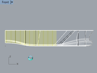 Fig. 64: Creating contours[/caption]